
First of all, congratulations if you ever downloaded Grapher: you are now one in a million! Honestly, a number this large had never even crossed my mind back when I was in the exciting process of releasing my very first Android application. After posting on the XDA Forums resulted in a crucial boost, another wave of growth came about when the academic year of 2015-2016 started. Words cannot express how grateful I am for this success as well as the support expressed by many lovely people, be it either by rating the app or by e-mailing me. Know that I truly appreciate and read every single review.
The domain coloring technique
In the midst of busily preparing for and starting my study abroad, I managed to push in an extra update that not only greatly expands Grapher Pro‘s complex analysis capabilities, but also showcases once again how beautiful mathematics can be. It takes us just one character to get started, namely the complex variable z:

So what exactly are we seeing here? This is nothing more than the identity function plotted onto the complex plane. Every point on the graph corresponds to an input z, whose real part re(z) is determined by the horizontal axis, and whose imaginary part im(z) is determined by the vertical axis. Next, applying any function f(z) gives us a new number with a certain magnitude and phase. The magnitude of this output then gets visualized as the brightness of the corresponding pixel, while the phase is translated to a color following this sequence from 0 to 2π: red – yellow – green – cyan – blue – magenta – red. It is important to note that the brightness periodically ‘wraps around’ from 100% to 0% at logarithmically spaced intervals (1, 2, 4, 8 …). This is useful because the values can get arbitrarily small and large: if we linearly mapped a magnitude in [0, 10] to a brightness in [0%, 100%], then smaller variations would not be discernible.
In the above example, the output equals the input as to get a sense of how this so-called domain coloring technique works. Real positive values are strictly red, while real negative values are strictly cyan (simply because cyan is the opposite of red in the RGB color space). Let’s see what adding an exponent does:

Trippy visuals aside, should we be surprised that a third-degree polynomial seems to run through the rainbow spectrum much faster, thus making every color appear three times? Not at all! The action of raising any complex number to the third power triples its phase, so for example, the output phase will be exactly 0 (= red) when the input phase is any multiple of 2π/3. Also, note how the concentric circles have become denser since the magnitude is now rising much faster as we move away from the origin.
Poles and zeros
Polynomials and rational functions lend themselves to an interesting side note. Consider A(z)=z^2-z-2 which has two real roots -1 and 2, and B(z)=z^2+1+i which has no real roots though (by the fundamental theorem of algebra) does have two complex roots near ±i. Dividing both polynomials to produce A(z)/B(z) gives:

The zeros with multiplicity 1 of this rational function can clearly be identified near -1 and 2 as they seem to “locally look like z“. Analogously for the complex poles which “locally look like 1/z“, we observe that the surrounding colors appear in a reversed order compared to the zeros. Moreover, the neighborhood of any pole or zero with multiplicity n will cycle through all colors n times. All of these observations are closely related to the residue theorem, which is yet another whole topic in and of itself that I shall not discuss further here.
A few pretty equations
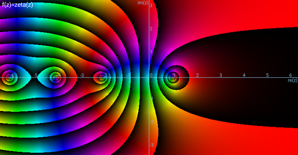
Now that we got our technical introduction out of the way, let’s get to the point of this article. I am convinced that complex functions serve not only as a tool for problem solving, but also as something that can be appreciated visually as a form of abstract art. Most formulas are discovered by just trying out functions and cascading them in random ways. However, even writing built-in functions without additives can already look stunning as exemplified by the Riemann zeta function:
I personally found that exponentiation is a powerful tool in creating surprising and often highly decorated results:
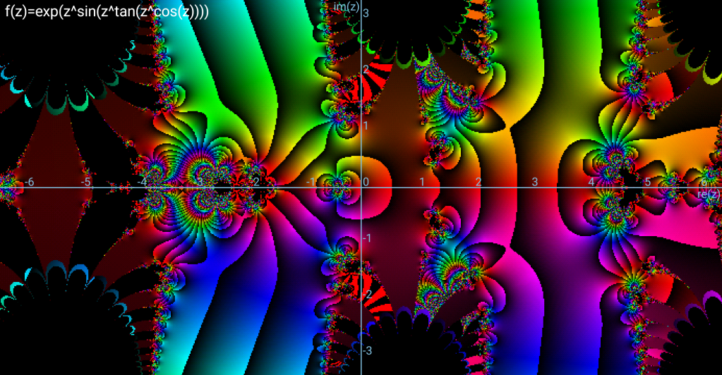
If these strongly remind you of fractals, you are definitely not alone. In fact, the Mandelbrot set could in principle be plotted directly using this method, although iterated functions are unfortunately not yet supported in Grapher. 😉
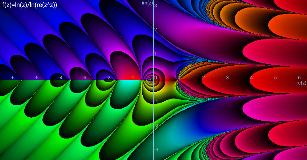
By utilizing the floor function that clamps input values to coordinates consisting of whole numbers, we can create mosaic-like patterns as well:
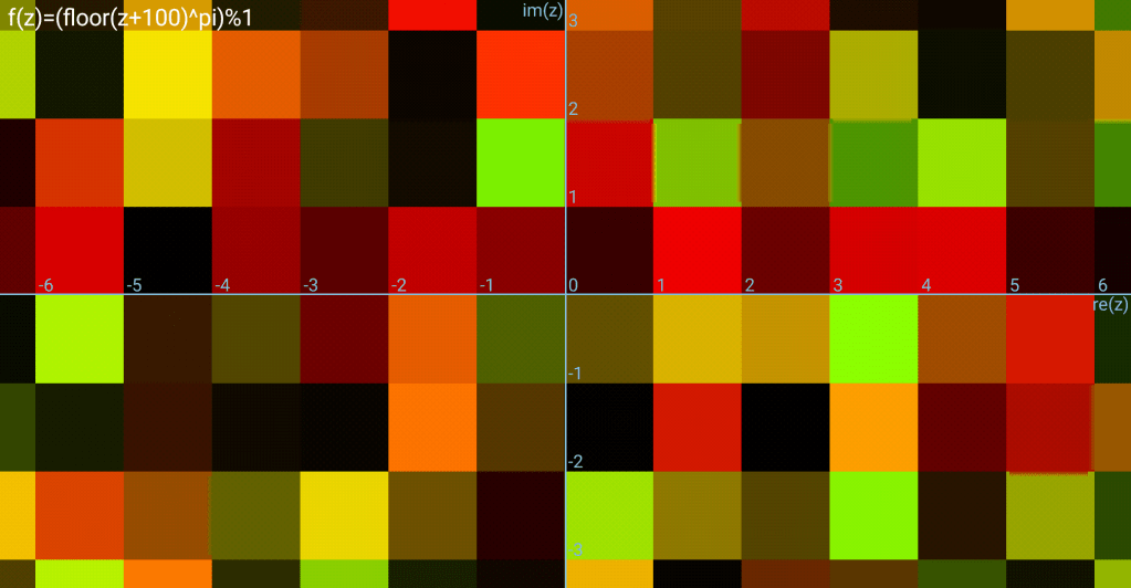
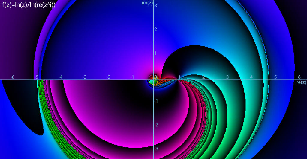
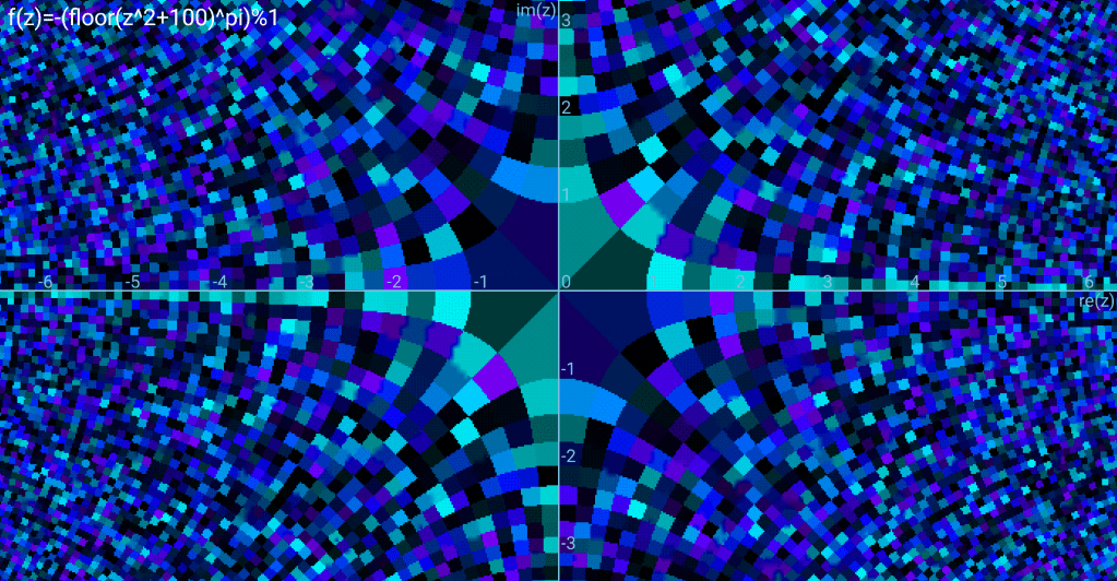
Here, raising to the power of π is just an ad-hoc way of pseudo-randomly generating colors. Things become even more interesting when you square z first, causing hyperbolas to emerge from the floor operation (these actually represent the constant real and imaginary lines of z^2 in some intermediate space):
So far, I have only touched the surface of what appears to be possible within the art of complex graphing. In any case, I hope to have introduced you to a magnificent new world. As I decided not to clutter this post with even more examples, I leave it up to you to experiment and share any other aesthetic discoveries you might make. Enjoy!
